Apache Spark

---

Getting Started with PySpark

Spark Data Types

About Spark 4.0 release including features like Spark Connect, etc.

About Spark Connect

---

The Core Philosophy

At its heart, Apache Spark is a distributed computing engine. It solves a physics problem: computers have limits (RAM, CPU). When your data exceeds those limits (Big Data), you cannot process it on one machine.

Spark allows you to treat a cluster of 100+ computers as if they were a single computer.

• In-Memory Processing: Unlike its predecessor Hadoop MapReduce (which wrote to disk after every step), Spark keeps data in RAM between steps, making it 100x faster for iterative logic.

• Unified Engine: It handles SQL, Streaming, and Machine Learning in one codebase.

---

The Architecture (The "How")

Spark uses a Master-Slave architecture.

1. The Driver (The Brain):

   • This is where your main() function runs (your Python script).

   • It converts your code into a "plan" (DAG).

   • It does not process the data itself; it tells the workers what to do.

2. The Cluster Manager:

   • The resource negotiator (e.g., YARN, Kubernetes, or Standalone).

   • The Driver asks it: "I need 50 CPUs and 200GB RAM."

3. The Executors (The Muscle):

   • These are processes running on the Worker Nodes.

   • They do the actual work (filtering, counting, aggregating).

   • They store data partitions in their local memory (RAM).

Jobs, Stages, and Tasks

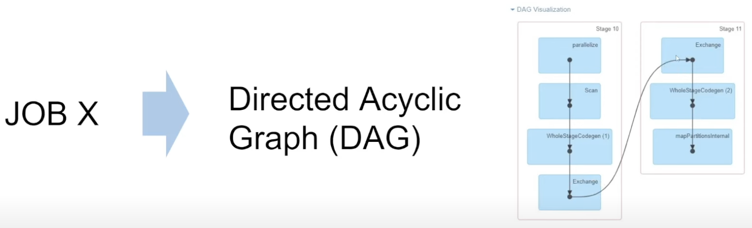
Every time we supply application to the Driver, it will split out application into 1 or more Jobs. Those Jobs can run in parallel, but more often they are run sequentially.

Each Job will have 1 or more Stages. The next Stage will ONLY start after the previous one is finished (exceptions can happen though). Inside each Stage we have many Tasks which can be run in parallel (as many as there are CPU cores).

The reasons why Stages happen sequentially is because Apache Spark tries to group all the data Transformations which do not require Data Shuffling (narrow transformations) into the same Stage.

As soon as the new Stage is required, it will be created. Hence, Data Shuffling is the boundary between Stages.

Each Job is represented by a DAG (Directed Acyclic Graph).

---

Primary Data Structures

1. RDD (Resilient Distributed Dataset)

• Concept: The "Assembly Language" of Spark. It is an immutable, distributed collection of objects.

• Pros: Total control.

• Cons: Slow (Python serialization overhead), no optimization engine.

• Verdict: Legacy. rarely used directly in modern PySpark 3.x+ unless you need low-level control.

2. DataFrame (The Modern Standard)

• Concept: A distributed table with named columns and a schema (like a Pandas DataFrame or SQL table).

• Pros:

  • Catalyst Optimizer: Spark automatically rewrites your code to be faster.

  • Tungsten: manages memory efficiently (off-heap).

• Verdict: Use this 99% of the time.

1. Dataset

About Dataset

The Dataset API is a fundamental part of Spark's architecture, and ignoring it gives an incomplete picture of the engine's capabilities, particularly for the Scala and Java ecosystems.

Even though Python users don't interact with it directly as a distinct type, it is actually the parent class of the DataFrame.

Here is the breakdown of the Dataset, why it was created, and the specific problem it solves.

The "Goldilocks" Solution

To understand Datasets, you have to look at the two options that existed before it (Spark 1.x):

1. RDDs (The "Safe" but Slow option):

   • Pros: You work with actual Java/Scala objects (Person, Transaction). You get Compile-Time Safety. If you try to access .nmae instead of .name, the code won't even compile.

   • Cons: Slow. Spark sees your objects as opaque "black boxes." It cannot optimize them. It relies on slow Java serialization.

2. DataFrames (The Fast but "Unsafe" option):

   • Pros: Blazing fast (Catalyst Optimizer + Tungsten).

   • Cons: You lose type safety. If you type df.select("naame") (typo), the code compiles fine. You only find out it’s broken when you run the job and it crashes (Runtime Error).

The Solution: The Dataset API (Spark 2.x+)

The Dataset is designed to be the "Best of Both Worlds."

• It has the Type Safety of RDDs.

• It has the Performance of DataFrames.

---

The Secret Sauce: Encoders

Why is the RDD slow? Because Java has to serialize the entire object to send it over the network.

Why is the Dataset fast? Because of Encoders.

An Encoder acts as a translator between your JVM objects (like a Person class) and Spark's internal binary format (Tungsten).

• Smart Serialization: Encoders map your object's fields directly to memory bytes.

• On-Demand Access: If you want to filter by age > 21, Spark doesn't need to deserialize the whole Person object. It knows exactly which bytes represent "age" and checks them directly in binary memory. RDDs cannot do this.

---

Dataset vs. DataFrame (The Relationship)

Technically, they are not two different things.

• In Scala/Java: A DataFrame is simply a type alias for a Dataset of generic Rows.

  • type DataFrame = Dataset[Row]

• In Python: Since Python is dynamically typed, it doesn't support the strict compile-time checks of Dataset[T](T for type). Therefore, PySpark only exposes the DataFrame (which behaves like Dataset[Row]).

The Dataset is the modern, strictly-typed API that powers Spark.

• Python users use it implicitly as Dataset[Row] (DataFrames).

• Scala users use it explicitly as Dataset[T] to get safety and speed simultaneously.

Visualizing the Hierarchy:

Feature	RDD	DataFrame	Dataset
Data Type	JVM Objects	Generic Row objects	Typed Objects (case class)
Safety	Compile-time	Runtime	Compile-time
Optimization	None	Catalyst	Catalyst
Primary Language	All	Python/R	Scala/Java

---

The Execution Model

This is the most critical concept for a developer.

Lazy Evaluation

Spark does nothing until you force it to.

1. Transformations (Lazy): "Instructions" on how to modify data (e.g., filter, map, join). Spark just remembers the "recipe." They are narrow or wide instructions that Spark records in the DAG.

2. Actions (Eager): Commands that demand a result (e.g., count, show, save). This triggers the actual computation. They force Spark to look at that DAG, optimize it, and send Tasks to the Executors to do the work

Why? If you filter a 1PB dataset and then ask for the top 5 rows, Spark optimizes the read to only scan what is necessary. It wouldn't know to do that if it executed every line immediately.

Wide vs. Narrow Transformations

• Narrow (Fast): Data processing happens independently on a single partition (e.g., filter, select). No data movement.

• Wide (Slow): Data must move between computers over the network. This is called a Shuffle. (e.g., groupBy, join, orderBy).

Why do we care about Data Shuffling?

• Shuffling is the process of redistributing data across partitions, and typically involves data exchange between executor nodes.

• Wide transformations require shuffling.

The beauty of Spark is that it processes data in-memory, which is another fundamental principle of Apache Spark and the reason why it’s so fast.

Whenever we’re talking about Data Shuffling, we need to take the data from the memory, save it to disk, send it over the network, then read it again to memory. Those operations are significantly slower than just in-memory processing.

Sometimes Data Shuffling can be avoided by not doing unnecessary sorts, optimizing joins, or filtering data early on. But generally, we shouldn’t go crazy about Data Shuffling, we should be aware of it, we should be aware when in our code it’s happening, but sometimes it cannot be avoided.

Shuffling in a nutshell:

• It requires saving data to the disk, sending it over network and reading data from the disk

• Data Shuffling can be very expensive

• Nevertheless, it’s often a “necessary evil”

The Result Destination

Actions usually result in one of two things:

• Returning data to the Driver: Commands like show(), collect(), or take(n) pull data from the Executors back to the "Brain" (the Driver).

  • Warning: Using collect() on a 1PB dataset will crash your Driver because it tries to fit all that data into the Driver's RAM.

• Writing to external storage: Commands like save() or write.parquet() move data from the Executors directly to a disk (like S3 or HDFS).

How Actions and Shuffling Interact

• When you call an Action, Spark looks at your code to see where the Wide Transformations (Shuffles) are.

• It breaks the Job into Stages based on those shuffles.

• It then executes the Tasks in parallel across your Executors.

---

PySpark Hands-On

Here is a complete modern workflow.

1. The Setup (SparkSession)

The SparkSession is your entry point.

from pyspark.sql import SparkSession
from pyspark.sql.functions import col, avg, desc

# Initialize the "Driver"
spark = SparkSession.builder \
    .appName("GroundUpExample") \
    .getOrCreate()

# Create a DataFrame (Simulating loading from a CSV/Parquet)
data = [
    ("Alice", "Engineering", 85000),
    ("Bob", "Marketing", 60000),
    ("Charlie", "Engineering", 90000),
    ("David", "Sales", 75000),
    ("Eve", "Engineering", 87000)
]
columns = ["Name", "Department", "Salary"]

df = spark.createDataFrame(data, columns)

2. Transformations (Defining the Plan)

Notice that running this code takes 0.01 seconds. No data has moved yet. We are just building the plan.

# Transformation 1: Filter
eng_df = df.filter(col("Department") == "Engineering")

# Transformation 2: Add a column (Bonus)
bonus_df = eng_df.withColumn("Bonus", col("Salary") * 0.10)

# Transformation 3: Aggregation (Wide Transformation - triggers Shuffle plan)
dept_stats = df.groupBy("Department").agg(
    avg("Salary").alias("AvgSalary"),
    count("Name").alias("EmployeeCount")
)

3. Actions (Executing the Plan)

Now, the Driver sends tasks to Executors, and data is processed.

# Action 1: Show results to console
print("Engineering Bonuses:")
bonus_df.show()

# Action 2: Collect data back to the Driver (Python list)
# WARNING: Do not do this on large datasets, or the Driver will crash (OOM).
results = dept_stats.collect() 

# Action 3: Save to disk (Parquet is best practice)
# bonus_df.write.mode("overwrite").parquet("/tmp/bonuses")

4. The SQL Interface

If you know SQL, you effectively know Spark.

# Register DataFrame as a temporary SQL view
df.createOrReplaceTempView("employees")

# Run pure SQL
sql_results = spark.sql("""
    SELECT Department, AVG(Salary) as AvgSalary
    FROM employees
    GROUP BY Department
    HAVING AVG(Salary) > 70000
""")

sql_results.show()

---

Advice on Best Practices

1. Avoid collect(): It drags all distributed data onto your single Driver machine and may end up crashing it. Use write() or show() instead.

2. Minimize Shuffles: groupBy and join are expensive. Filter your data before you join it.

3. Use DataFrames: Avoid RDDs (sc.parallelize, map, reduceByKey) unless you are writing a custom low-level library. DataFrames are significantly faster due to the Catalyst Optimizer.

4. Partitioning Strategy

   Writing data efficiently is just as important as reading it.

   • Partition your data on disk: When saving files, use .partitionBy("column_name"). This allows Spark to skip reading entire folders of data if your query filters by that column.

   • Avoid "Small File" syndrome: Aim for partition sizes of 128MB to 256MB. If your files are too small (e.g., 1KB), Spark spends more time opening files than actually processing data.

5. Broadcast Joins (The Shuffle Killer)

   Minimizing shuffles—this is the most effective way to do it.

   • Small + Large Join: If you are joining a massive table (1TB) with a small lookup table (10MB), use a Broadcast Join.

   • Why? Spark sends a copy of the small table to every executor, so no data from the big table needs to move across the network.

     Code Tip: from pyspark.sql.functions import broadcast; df_large.join(broadcast(df_small), "id")

6. Early Filtering (Predicate Pushdown)

   1. Filter Early, Filter Often: Always place your .filter() or .where() clauses as close to the data source as possible.

   2. Pushdown: If you use formats like Parquet, Spark can "push" your filter down to the storage layer, meaning it only pulls the specific rows it needs into memory.

7. Caching and Persisting

   1. Reuse Data: If you plan to use the same DataFrame in three different actions, use .cache().

   2. Don't Over-Cache: Caching takes up RAM. If you cache everything, you’ll run out of memory for the actual processing. Remember to .unpersist() when you are done.

"Checklist" section. Before you submit a Spark job, you should ask:

1. Did I filter the data as early as possible?

2. Is my join using a broadcast if one side is small?

3. Am I writing to an External Table to prevent accidental deletion?

---

Spark Shell

What is the Spark Shell?

The Spark Shell is an interactive playground for Apache Spark. Technically, it is a REPL (Read-Eval-Print Loop) environment that allows you to write Spark code and see the results immediately, line-by-line, without needing to compile a full application or write a complex script file.

Think of it as the "command line" for your cluster.

---

Key Features

• Pre-configured Environment: When you launch the shell, it automatically creates the two most important objects for you:

  • spark: An active SparkSession object.

  • sc: An active SparkContext object.

  • You don't need to write the setup code (e.g., SparkSession.builder...)—it's just there.

• Immediate Feedback: You type a transformation, hit Enter, and can immediately inspect the schema or show the data.

• Language Support:

  • PySpark Shell: For Python (Launched via pyspark).

  • Spark Shell: For Scala (Launched via spark-shell).

---

How to Use It (Python Perspective)

To start it, you simply open your terminal and type:

$ pyspark

If you have IPython installed, it will launch an enhanced shell with color coding and auto-completion. You will see a welcome banner that looks like this:

Welcome to
      ____              __
     / __/__  ___ _____/ /__
    _\ \/ _ \/ _ `/ __/  '_/
   /__ / .__/\_,_/_/ /_/\_\   version 4.0.0
      /_/

Using Python version 3.10.x
SparkSession available as 'spark'.
>>>

Now you can immediately start analyzing data:

>>> df = spark.read.csv("data.csv", header=True)
>>> df.printSchema()
root
 |-- name: string (nullable = true)
 |-- age: string (nullable = true)

>>> df.count()
150

---

When to Use It

Even in a modern workflow, the Shell is useful for:

1. Prototyping: "Will this regex filter work?" (Test it in 10 seconds in the shell before adding it to your production code).

2. Cluster Debugging: If a job is failing, you can SSH into the cluster, open the shell, and try to read the file manually to see if it's a permissions issue or corrupt data.

3. Learning: It is the fastest way to memorize the API.

Modern Context: Shell vs. Notebooks

If you use tools like Jupyter Notebooks, Databricks, or Zeppelin, you are effectively using a "Spark Shell with a GUI."

• The Shell: Text-only, runs in a terminal.

• Notebooks: Web-based, supports charts/graphs, but connects to a Spark Shell session in the background.

---

SparkSQL

What is Spark SQL?

Spark SQL is the module of Apache Spark that handles structured data.

It is often misunderstood as just "a way to run SQL queries." In reality, it is the kernel of modern Spark. Whether you are writing Python DataFrames, streaming data with Structured Streaming, or doing Machine Learning, you are actually running on top of the Spark SQL engine.

It serves two main roles:

1. The API: It lets you run ANSI-standard SQL queries (like SELECT * FROM table) on your data.

2. The Engine: It powers the DataFrame API, ensuring that Python code is optimized just as heavily as raw SQL.

---

The "Rosetta Stone" of Spark

Spark SQL allows you to seamlessly mix different languages and data sources in a single application.

• Unified Data Access: You can read a JSON file, join it with a Hive table, and write the result to a Parquet folder—all in one query.

• Integrated Logic: You can start with a Python DataFrame, register it as a temporary table, run a complex SQL query on it, and get the result back as a Python DataFrame.

---

How to Use It: The Two Interfaces

One of the most powerful concepts to grasp is that Spark SQL and DataFrames are the same thing.

When you write Python code, Spark translates it into a "SQL Plan" behind the scenes. This means there is zero performance difference between writing a SQL query string and writing PySpark code.

Scenario: Find the average salary of "Engineers."

Option A: The PySpark Way (Programmatic)

df.filter(col("dept") == "Engineering") \
  .groupBy("dept") \
  .agg(avg("salary")) \
  .show()

Option B: The Spark SQL Way (Declarative)

# 1. Register the DataFrame as a view so SQL can see it
df.createOrReplaceTempView("employees")

# 2. Run pure SQL
spark.sql("""
    SELECT dept, AVG(salary)
    FROM employees
    WHERE dept = 'Engineering'
    GROUP BY dept
""").show()

Result: Both generate the exact same Catalyst Plan and run at the exact same speed.

---

The Hive Metastore (The "Catalog")

Spark SQL allows you to create a permanent "Data Warehouse" structure over your files using the Hive Metastore.

• Without Metastore: You always have to remember where your files are:

  spark.read.parquet("s3://bucket/data/2024/sales/")

• With Metastore: You define a table once, and Spark remembers the location and schema.

  spark.sql("SELECT * FROM production.sales")

Managed vs. Unmanaged Tables:

• Managed Table: Spark manages both the data (files) and the metadata. If you DROP TABLE, the files are deleted.

• External (Unmanaged) Table: Spark manages only the metadata. If you DROP TABLE, the files remain in S3/HDFS.

Why the Metastore is Essential

• Abstraction: It allows data engineers to change file locations or storage tiers (e.g., moving from one S3 bucket to another) without breaking the downstream SQL queries used by data analysts.

• Schema Enforcement: The Metastore acts as the single source of truth for column names and data types, preventing "schema drift" where different scripts interpret the same file differently.

• Discovery: It enables tools like PowerBI, Tableau, or Presto to "see" your Spark data because they query the Metastore to find out what tables exist.

The "Execution" Connection

To tie this back to your the previous information about Actions:

• When you run spark.sql("SELECT * FROM sales"), Spark first goes to the Hive Metastore to look up the file path.

• It then builds the DAG based on the files it finds at that path.

• The actual reading of the data only happens once you trigger an Action (like .show()).

Key Takeaway: The Metastore is the "Phonebook" of your data. You don't need to know where your friends live (the file path); you just need to know their name (the table name).

Managed vs. Unmanaged: The "Safety" Factor

This is the part that usually catches developers off guard. Understanding this prevents accidental data loss.

Feature	Managed Table	External (Unmanaged) Table
Control	Spark/Hive owns the data.	You own the data.
Storage Location	Typically in a default "warehouse" folder.	Any path you specify (S3/HDFS/Azure Blob).
DROP TABLE	Deletes the metadata AND the physical files.	Deletes the metadata ONLY. Files stay safe.
Best Practice	Good for temporary or internal sandbox tables.	Standard for production. Ensures data persists even if the table is recreated.

To clarify, the Hive Metastore itself is essential and used in almost every production Spark environment, but Managed Tables (a specific way of using the Metastore) are often avoided in production because they carry the risk of accidental data loss.

Why "Managed Tables" are the Risk

The confusion usually stems from the two types of tables the Metastore tracks:

1. Managed Tables (The "Risky" Choice)

• How they work: Spark "owns" both the entry in the Metastore and the physical files on the disk.

• The Danger: If a developer runs DROP TABLE sales_data, Spark assumes you want to delete everything. It wipes the metadata from the Metastore and permanently deletes the files from S3/HDFS.

• Production Use: Rarely used for primary data. They are mostly used for temporary "scratchpad" work or internal staging where the data is easily replaceable.

2. External Tables (The "Production" Choice)

• How they work: You tell the Metastore, "Here is a table called sales, but the data actually lives over in this S3 folder".

• The Safety: If you run DROP TABLE sales, Spark only deletes the "shortcut" in the Metastore. Your actual data files remain untouched.

• Production Use: This is the industry standard. It ensures that if someone accidentally deletes a table definition, you can simply recreate the table pointing back to the same folder, and your data is back.

---

Modern Features (Spark 4.0+)

A. ANSI Compliance (Strict Mode)

In the past, Spark was "lenient." If you inserted a String into an Integer column, it might just turn it into NULL.

Spark 4.0 runs in ANSI Mode by default.

• Behavior: It throws explicit errors for overflow or type mismatches (similar to Postgres or Snowflake).

• Benefit: Keeps your data clean and prevents silent data corruption.

B. The VARIANT Data Type

If you work with semi-structured data (like raw JSON logs), Spark SQL now has a VARIANT type.

• Old Way: You had to define a strict schema (struct<name:string, age:int>) to read JSON efficiently.

• New Way: You load it as VARIANT. Spark figures out the structure on the fly but stores it in a binary, optimized format that is much faster to query than raw strings.

---

More about Spark Transformations

More about lazy evaluation, transformations, and actions

In Apache Spark, a transformation is a set of instructions used to modify or transform a dataset (DataFrame/RDD) into a new one.

The defining characteristic of transformations is that they are lazy.

• Lazy Evaluation: When you tell Spark to filter, join, or select, it does not immediately process the data.

• The Plan: Instead, it adds your instruction to a "logical plan" (a Directed Acyclic Graph, or DAG).

• The Trigger: Nothing happens until you call an Action (like count(), show(), or write()).

---

The Two Types of Transformations

Understanding the difference between Narrow and Wide transformations is the single most important factor in optimizing Spark performance.

1. Narrow Transformations (Fast)

In a narrow transformation, the data required to compute the records in a single partition resides in at most one partition of the parent dataset.

• Behavior: No data movement is required across the network. The work happens "locally" on each executor (RAM).

• Examples:

  • filter(): "Keep only rows where age > 21." (Can be done by checking one row at a time).

  • select(): "Keep only column A and B."

  • withColumn(): "Add a new column based on existing data."

  • drop(): "Remove a column."

2. Wide Transformations (Slow / "The Shuffle")

In a wide transformation, the data required to compute the records in a single partition may reside in many partitions of the parent dataset.

• Behavior: This triggers a Shuffle. Data must be written to disk, sent over the network to other nodes, and reorganized so that related records end up on the same machine.

• Cost: This is expensive (Disk I/O + Network I/O + Serialization).

• Examples:

  • groupBy(): "Group all 'Engineering' employees together." (They might be scattered across 50 different nodes).

  • join(): "Match rows from Table A with Table B."

  • distinct(): "Find unique values."

  • orderBy(): "Sort the entire dataset."

---

Visualizing the Process

Imagine you are organizing a deck of cards scattered across 4 different rooms (partitions).

1. Narrow (Filter): "Remove all Jokers."

   • You can go into each room and throw away Jokers independently. You don't need to talk to the other rooms. This is fast.

2. Wide (GroupBy): "Put all Aces in one pile, all Kings in another."

   • You cannot do this in isolation. You have to take the Aces from Room 1, walk them over to Room 2, take the Kings from Room 2, walk them to Room 3, etc. This is the Shuffle.

---

Code Examples (PySpark)

Here is how these look in code.

from pyspark.sql import SparkSession
from pyspark.sql.functions import col

spark = SparkSession.builder.appName("Transformations").getOrCreate()

# Create a sample DataFrame
df = spark.createDataFrame([
    ("Alice", "Sales", 5000),
    ("Bob", "Eng", 7000),
    ("Charlie", "Sales", 6000)
], ["Name", "Dept", "Salary"])

# --- Narrow Transformation ---
# Spark notes this down but executes NOTHING yet.
filtered_df = df.filter(col("Salary") > 5500)

# --- Wide Transformation ---
# Spark notes this down. It knows it will need to Shuffle data later.
grouped_df = df.groupBy("Dept").count()

# --- ACTION (The Trigger) ---
# NOW, Spark looks at the plan, optimizes it, and runs the job.
grouped_df.show()

Summary Table

Feature	Narrow Transformation	Wide Transformation
Data Movement	None (In-memory, local)	Shuffle (Network + Disk I/O)
Dependency	1-to-1 (One input partition → One output partition)	Many-to-1 (Many input partitions → One output partition)
Speed	Very Fast	Slow (Bottleneck)
Examples	filter, select, map	groupBy, join, orderBy, repartition

---

Catalyst Optimizer

The Catalyst Optimizer is the "brain" behind Spark SQL and DataFrames. It is the reason why you can write "inefficient" code in Python, yet Spark still executes it efficiently.

What Does Catalyst Do?

When you write code like df.filter(...).join(...), you are just giving Spark a "wish list" of what you want. You aren't telling it how to do it.

Catalyst takes your code and moves through four distinct phases to produce the most efficient execution plan possible.

---

The 4 Phases of Catalyst Optimization

1. Analysis (The "Spell Checker")

• Input: Your code (Unresolved Logical Plan).

• Action: Spark checks if the table names and column names actually exist.

  • Example: If you type df.select("naame") but the column is name, Catalyst flags the error here.

• Output: Logical Plan (Resolved).

2. Logical Optimization (The "Strategist")

This is where the magic happens. Catalyst applies standard rule-based optimizations to rearrange your logic without changing the result.

• Predicate Pushdown:

  • You wrote: Load all data -> Join Table A and B -> Filter for year = 2024.

  • Catalyst changes it to: Filter Table A for year = 2024 -> Load only that data -> Join.

  • Benefit: Drastically reduces the data sent to the Join (Wide Transformation).

• Constant Folding:

  • You wrote: filter(col("age") > 10 + 5)

  • Catalyst changes it to: filter(col("age") > 15) so it doesn't calculate 10+5 for every billion rows.

• Column Pruning:

  • You wrote: Load a 100-column CSV -> Select only "Name".

  • Catalyst changes it to: Only scan the "Name" column from the file (if the file format, like Parquet, supports it).

3. Physical Planning (The "Tactician")

Now Catalyst knows what to do, but it needs to decide how to do it on the hardware. It generates multiple plans and compares their "cost" (estimated time/resources).

• Join Selection:

  • Should it use a Sort Merge Join (good for two massive tables)?

  • Or a Broadcast Hash Join (good if one table is tiny)?

  • Decision: If one table is < 10MB, it chooses Broadcast (much faster).

4. Code Generation (The "Translator")

• Project Tungsten: Once the best physical plan is selected, Spark generates optimized Java bytecode to run on the executors.

• Whole-Stage Code Generation: Instead of calling a function for every row (which is slow), it collapses the entire query into a single optimized function (simulating a "hand-written" loop).

Diagram: Journey of a query

---

Visualizing the "Before and After"

Imagine you write this query:

users.join(transactions, "user_id") \
     .filter(users.country == "US") \
     .select("transactions.amount")

Without Catalyst (Naive Execution):

1. Read ALL users (1 Billion rows).

2. Read ALL transactions (10 Billion rows).

3. Shuffle both massive datasets across the network to Join them.

4. Scan the result and throw away everyone not from the "US".

5. Throw away all columns except "amount".

With Catalyst (Optimized Execution):

1. Predicate Pushdown: Read only users where country = "US" (maybe 50 million rows).

2. Column Pruning: Read only user_id and amount from transactions.

3. Join: Join the smaller filtered lists.

How to See It Yourself

You can see Catalyst's work by using the .explain() method in PySpark.

df = spark.read.parquet("data.parquet")
result = df.filter("id > 100").select("name")

# This prints the plan to the console
result.explain(True)

You will see the output broken down into Parsed Logical Plan, Analyzed Logical Plan, Optimized Logical Plan, and Physical Plan.

---

What is Project Tungsten?

If Catalyst is the "Brain" (optimizing the logical plan), Tungsten is the "Muscle" (optimizing the physical execution).

In the early days of Spark, the bottleneck was often I/O (network and disk speed). As hardware improved (faster SSDs, 10Gbps networks), the bottleneck shifted to the CPU and Memory. Spark was spending too much time waiting for the Java Virtual Machine (JVM) to manage objects.

Project Tungsten was introduced to solve this by bypassing the JVM's standard memory management and getting "closer to the metal."

---

The 3 Key Features of Tungsten

1. Explicit Memory Management (Off-Heap Memory)

• The Problem: The JVM is great for general applications, but bad for Big Data.

  • Object Overhead: A simple 4-byte string like "abcd" might take 48 bytes of RAM in Java due to object headers and metadata.

  • Garbage Collection (GC): When you have millions of objects, the JVM pauses to clean up memory ("GC Pauses"), which kills performance.

• The Tungsten Solution:

  • Spark manages its own memory explicitly, allocating raw binary memory blocks (off-heap) instead of creating Java objects.

  • It uses the sun.misc.Unsafe API (the same tricks C++ developers use) to manipulate raw bytes.

  • Result: No GC pauses for data storage, and significantly denser memory usage.

2. Cache-Aware Computation

• The Problem: Modern CPUs are incredibly fast, but fetching data from RAM is slow relative to the CPU speed. If the CPU has to wait for data, it sits idle (L1/L2/L3 cache misses).

• The Tungsten Solution:

  • Tungsten designs algorithms and data structures to be "cache-friendly."

  • It arranges data in memory so that it flows smoothly into the CPU's L1/L2 cache, minimizing the time the CPU spends waiting.

3. Whole-Stage Code Generation (WSCG)

• The Problem: In standard Spark (pre-Tungsten), every operator (Filter, Select, Map) was a function call.

  • When processing 1 billion rows, calling a filter() function 1 billion times creates massive CPU overhead (virtual function calls).

• The Tungsten Solution:

  • Tungsten looks at the entire query plan and compiles it into a single function of optimized Java bytecode on the fly (using a library called Janino).

  • It effectively writes a while loop by hand for you.

Visualizing Code Generation:

• Before Tungsten (Volcano Model):

  # Conceptually, Spark did this:
  for row in data:
     result1 = filter_function(row)
     result2 = project_function(result1)
     emit(result2)

  (Lots of function calls and passing data between steps)

• After Tungsten (WSCG):

  // Tungsten generates and compiles this actual bytecode:
  while (rows.hasNext()) {
     Row row = rows.next();
     if (row.age > 21) {   // Filter inlined
        // Project inlined
        // No function calls!
        output.append(row.name); 
     }
  }

  (One tight loop, extremely fast)

---

Summary: Catalyst vs. Tungsten

Feature	Catalyst Optimizer	Project Tungsten
Role	The Strategist (Logic)	The Muscle (Hardware)
Focus	"What is the smartest way to run this query?"	"How can we run this plan as fast as C++?"
Key Tech	Predicate Pushdown, Join Reordering	Off-Heap Memory, Code Generation, CPU Cache Optimization
User Action	Use DataFrames/SQL to enable it.	Automatic (enabled by default since Spark 2.x).

---

Joins

This is the most critical performance topic in Spark. Understanding join strategies separates a novice from an expert.

Spark has about 5 different ways to join data, but in 99% of production scenarios, you only care about two: Broadcast Hash Join and Sort Merge Join.

---

1. The Strategies

A. Broadcast Hash Join (The "Ferrari")

• Scenario: Joining a Large Table (Fact) with a Tiny Table (Dimension).

• Mechanism: Spark broadcasts (copies) the entire tiny table to every Executor's memory. The large table does not move (no shuffle). Each executor joins its slice of the big table with the local copy of the small table.

• Pros: Extremely fast (No network shuffle for the big data).

• Cons: If the "tiny" table is actually huge, you will crash the executors with Out-Of-Memory (OOM) errors.

B. Sort Merge Join (The "Workhorse")

• Scenario: Joining two Large Tables.

• Mechanism:

  1. Shuffle: Both tables are shuffled so that matching keys (e.g., user_id) land on the same partition.

  2. Sort: Both sides are sorted by the join key.

  3. Merge: Spark iterates through both sorted lists to find matches (like zippering two lists).

• Pros: Robust. Can handle petabytes of data without OOM (because it can spill to disk).

• Cons: Expensive (Heavy CPU for sorting, Heavy Network for shuffling).

C. Shuffle Hash Join (The "Specialist")

• Scenario: Large tables, but one is smaller than the other (and fits in memory), and you want to avoid sorting.

• Mechanism: Shuffles data, but instead of sorting, it builds a Hash Map of the smaller side in memory.

• Status: Often disabled by default in favor of Sort Merge, but can be forced for specific optimizations.

---

2. Tuning Parameters

Broadcast Threshold

How does Spark decide when to use Broadcast vs. Sort Merge?

• Config: spark.sql.autoBroadcastJoinThreshold

• Default: 10 MB

• Usage: If a table is smaller than 10MB, Spark automatically broadcasts it.

• Tuning: In modern clusters with lots of RAM, you often bump this up to 100MB or 1GB to force faster joins.

  spark.conf.set("spark.sql.autoBroadcastJoinThreshold", "104857600") # 100 MB

Spark Parallelism (Shuffle Partitions)

This controls how many partitions are created after a wide transformation (like a Join).

• Config: spark.sql.shuffle.partitions

• Default: 200

• The Trap:

  • For huge data (TB), 200 is too low (partitions will be massive, causing OOM).

  • For tiny data, 200 is too high (lots of tiny files/overhead).

• Rule of Thumb: Aim for partitions of ~128MB - 200MB.

---

3. Using .explain() to Optimize

You use df.explain() to check if Spark is picking the strategy you want.

Example 1: Detecting a Sort Merge Join (Slow)

df_joined = big_table.join(medium_table, "id")
df_joined.explain()

Output Look-for:

SortMergeJoin [id], [id], Inner

(This means Spark thinks medium_table is too big to broadcast.)

The Fix (Broadcasting Hints):

If you know medium_table fits in RAM (e.g., it has 500k rows but Spark's size estimation is wrong), you can force a broadcast using a hint.

from pyspark.sql.functions import broadcast

# "Trust me, Spark, this fits in memory."
df_optimized = big_table.join(broadcast(medium_table), "id")
df_optimized.explain()

Output Look-for:

BroadcastHashJoin [id], [id], Inner, BuildRight

(Success! You just skipped the shuffle.)

---

Adaptive Query Execution (AQE)

New in Spark 3.x, Default in 4.0.

AQE is a game-changer because it allows Spark to fix its plans at runtime.

A. Dynamically Switching Join Strategies

• Scenario: You join Table A and Table B. Spark estimates Table B is 100MB (too big to broadcast), so it plans a Sort Merge Join.

• Reality: You filtered Table B (WHERE id > 1000), and at runtime, it shrinks to only 2MB.

• AQE Action: Spark pauses, realizes the data is small, and converts the plan to a Broadcast Join on the fly.

B. Optimizing Skew Join

Data Skew is when one key has massive amounts of data (e.g., user_id = null or a "popular item").

• The Problem: In a normal join, the partition handling the "popular key" will take 5 hours while others take 5 minutes. The job waits for the straggler.

• AQE Solution:

  1. Spark detects that one partition is suspiciously large.

  2. It splits that large partition into smaller sub-partitions.

  3. It duplicates the matching data from the other table.

  4. It processes these splits in parallel.

How to enable AQE (if not on by default):

spark.conf.set("spark.sql.adaptive.enabled", "true")
spark.conf.set("spark.sql.adaptive.skewJoin.enabled", "true")

Summary Checklist for Joins

1. Check the Plan: Use .explain() to see if you have SortMergeJoin or BroadcastHashJoin.

2. Broadcast Small Tables: Use the broadcast() hint or increase the autoBroadcastJoinThreshold if a table fits in memory.

3. Handle Skew: Ensure AQE is enabled to automatically fix skewed partitions.

4. Check Partition Counts: If your join is slow, check if spark.sql.shuffle.partitions (200) needs to be increased.

---

repartition() and coalesce()

repartition(n): The Heavy Lifter

What it does: It can increase or decrease the number of partitions.

How it works: It performs a Full Shuffle. It redistributes data evenly across the network to ensure that all partitions are roughly the same size.

• Mechanism: It creates a hash of rows and sends data across the network to new nodes. It completely rewrites the data distribution.

• Cost: High. (Requires Network I/O, Disk I/O, and Serialization).

• When to use it:

  • Increasing Parallelism: You loaded a compressed 1GB file (which Spark might read as 1 partition). You want to process it with 100 cores. You call df.repartition(100).

  • Fixing Data Skew: If Partition 1 has 1 million rows and Partition 2 has 10 rows, repartition will balance them so both have ~500,000.

  • Filtering: After a heavy filter (e.g., removing 90% of data), your partitions might be empty or uneven. repartition fixes this layout.

---

coalesce(n): The Efficient Merger

What it does: It can only decrease the number of partitions.

How it works: It avoids a full shuffle. Instead of moving data across the network, it simply "stitches" existing local partitions together.

• Mechanism: If you have partitions 1, 2, 3, 4 on one machine, and you coalesce(2), it essentially says "Okay, 1 & 2 are now Partition A; 3 & 4 are Partition B." No data moves between machines.

• Cost: Low. (Local metadata operation).

• When to use it:

  • Final Write: You processed data using 1,000 partitions for speed, but you don't want to write 1,000 tiny files to S3. You use df.coalesce(10).write... to produce 10 clean output files.

  • Limit: If you ask to increase partitions (e.g., go from 10 to 100) using coalesce(100), Spark will simply ignore you and keep 10.

---

The Visual Analogy

Imagine you have 4 stacks of cards on a table.

• Repartition (4 stacks $\rightarrow$ 2 stacks):

  • You pick up all the cards from all 4 stacks, shuffle them thoroughly, and deal them out into 2 perfectly even new stacks.

  • Result: Perfectly balanced, but takes a long time.

• Coalesce (4 stacks $\rightarrow$ 2 stacks):

  • You take Stack 1 and place it on top of Stack 2. You take Stack 3 and place it on top of Stack 4.

  • Result: Fast, but the resulting stacks might be uneven (if Stack 1 was huge and Stack 2 was tiny, the new combined stack is massive).

---

Comparison

Feature	repartition(n)	coalesce(n)
Direction	Increase or Decrease	Decrease Only
Shuffle	Yes (Full Shuffle)	No (Local Merge)
Balancing	Perfect (Round Robin/Hash)	Imperfect (Depends on upstream size)
Performance	Slower (Network/Disk heavy)	Faster (Metadata only)
Primary Use	Fixing Skew / Increasing Parallelism	Reducing file count for output

---

The "Coalesce Trap" (Pro Tip)

There is a dangerous side effect of coalesce() that trips up many developers.

Because coalesce is optimized to merge partitions, Spark's optimizer might push the partition reduction upstream to the source.

The Scenario:

You have a massive job. You want to process it in parallel (100 cores), but write only 1 file at the end.

# DANGEROUS CODE
df = spark.read.parquet("/data/huge_file")
df = df.filter(...) # Heavy logic
df.coalesce(1).write.csv("/output") 

What happens:

Spark sees coalesce(1) and thinks, "Oh, you only want 1 partition? I'll just use 1 core from the very beginning!"

• Result: Your entire heavy logic runs on 1 single core, and the job takes hours instead of minutes.

The Fix:

Force a shuffle using repartition if you need parallel processing before the final write.

# SAFE CODE
df = spark.read.parquet("/data/huge_file")
df = df.repartition(100) # Force 100 parallel cores
df = df.filter(...)      # Logic runs fast on 100 cores
df.coalesce(1).write.csv("/output") # Combine at the very end

---

Optimizations that Spark does vs what a user can do

What can a user do to optimize Spark workflows:

• Use Parquet or Delta files instead of CSV (don’t use CSV if possible)

• Avoid expensive operations like sort()

• Minimize volume of data

• Cache / persist dataframes

• Repartition/coalesce

• Avoid UDFs

• Partitioning / Indexing data

• Bucketing

• Optimize cluster

• and so many more

What Spark already does for us:

• Catalyst Optimizer handles logical and physical query plan optimizations

• Tungsten provides low-level optimizations and code generation techniques to improve overall performance

• AQE dynamically adjusts query execution based on runtime conditions

---

Data Modeling in Spark

When we talk about "Data Modeling" in a traditional database (like PostgreSQL), we talk about Normalization (3NF), Foreign Keys, and reducing redundancy.

In Spark (and Big Data), the goal is the opposite. We denormalize data to avoid joins, and we obsess over File Layout.

The Golden Rule of Spark Data Modeling: "How you save your files determines how fast you can read them."

---

1. Partitioning (The Directory Structure)

This is the single most important decision you will make. Partitioning breaks your massive dataset into smaller, manageable chunks based on a specific column.

• The Concept: Instead of scanning a 10TB file to find data for "2024," you tell Spark to organize the files into folders by year.

• The Mechanism: This creates a Hive-style directory structure.

Bad Modeling (Flat):

/data/sales.parquet (1 massive file. Spark must scan the whole thing to find anything.)

Good Modeling (Partitioned):

/data/sales/
    ├── year=2023/
    │   ├── month=01/
    │   │   └── part-0001.snappy.parquet
    │   └── month=02/
    └── year=2024/
        ├── month=01/
        └── month=02/

The Code:

df.write.partitionBy("year", "month").parquet("/data/sales")

The "Goldilocks" Trap (Cardinality)

You must choose your partition column carefully.

• Too Few Partitions (Low Cardinality): Partitioning by Gender (only 2 folders). The files are still too big.

• Too Many Partitions (High Cardinality): Partitioning by UserID (1 million folders). This creates the Small File Problem.

  • Why it kills performance: The NameNode (metadata server) crashes trying to manage millions of tiny files. Opening a file takes longer than reading the data inside it.

• Just Right: Dates (year, month, date) or broad categories (region, department).

---

2. File Formats (Row vs. Column)

Spark is optimized for Columnar Storage.

• Row-Oriented (CSV, JSON, Avro):

  • Good for: Writing data one row at a time (e.g., Streaming landing zone).

  • Bad for: Analytics. To calculate "Average Salary", the computer has to read the "Name" and "Address" of every person just to skip over them.

• Column-Oriented (Parquet, ORC):

  • Good for: Analytics. All "Salaries" are stored side-by-side in bytes.

  • Projection Pushdown: Spark can read only the Salary column bytes and ignore the rest of the file entirely.

Recommendation: Always convert your raw data (JSON/CSV) into Parquet (or Delta/Iceberg) for the "Silver/Gold" layers of your data lake.

---

3. File Sizing (The 128MB Rule)

Spark works best when files are roughly 128MB to 1GB in size.

• If you have 10,000 files that are 1KB each, Spark will be incredibly slow (metadata overhead).

• If you have 1 file that is 100GB, you lose parallelism (only one core can read it at a time).

The Fix:

If you filtered a large dataset and are about to write it out, check how many partitions you have in RAM.

# Bad: Writing 200 tiny files
df.write.parquet("/output") 

# Good: Combine them into fewer, larger files before writing
df.coalesce(5).write.parquet("/output")

---

4. Bucketing (Sorting within Partitions)

Note: This is an advanced optimization.

Partitioning creates folders. Bucketing creates specific files inside those folders, hashed by a key.

• Use Case: If you constantly join two massive tables on user_id.

• Strategy: You "bucket" both tables by user_id into, say, 50 buckets.

• Benefit: Spark knows that user_id=100 is definitely in Bucket 5 for both tables. It can join them without a Shuffle. This is called a Sort-Merge Join.

---

5. The Modern Standard: Table Formats (Delta Lake / Iceberg)

In Spark 4.0, you rarely write raw Parquet anymore. You use a "Table Format" like Delta Lake.

These wrap your Parquet files in a transaction log (_delta_log).

1. ACID Transactions: You can update/delete rows without rewriting the whole table.

2. Time Travel: You can query SELECT * FROM table VERSION AS OF 5.

3. Z-Ordering: A technique to "sort" data along multiple dimensions (e.g., sort by both Year and Country) to make file skipping extremely efficient.

Modern Code Example:

# Create a Delta table (automatically manages the transaction log)
df.write.format("delta").save("/data/sales_delta")

# Optimize the layout (Compact small files + Z-Order sort)
from delta.tables import *
deltaTable = DeltaTable.forPath(spark, "/data/sales_delta")
deltaTable.optimize().executeCompaction() 

Summary of Data Modeling

1. Format: Use Parquet (or Delta).

2. Partitioning: Folder structure based on query patterns (usually Time). Avoid high cardinality.

3. Sizing: Aim for 128MB files.

4. Schema: Denormalize. Arrays and Structs are okay; Joins are expensive.

---

What is a UDF (User Defined Function)?

A UDF is a feature that allows you to write your own custom logic in Python (or Scala/Java) and apply it to a Spark DataFrame, row by row.

It is effectively a way to say: "Spark, your built-in functions (like avg, col, substring) aren't enough for me. Here is a custom Python function I wrote; please run this on every single row of my 10TB dataset."

Code Example:

# A simple Python function
def reverse_string(s):
    return s[::-1]

# Registering it as a UDF
from pyspark.sql.functions import udf
from pyspark.sql.types import StringType

reverse_udf = udf(reverse_string, StringType())

# Using it
df.withColumn("reversed_name", reverse_udf("Name"))

---

Why Are They Not Recommended? (The "Python Trap")

In PySpark, standard Python UDFs are a performance killer. They are often called the "Black Box" of Spark optimization. Here is why:

1. The Serialization Bottleneck ("The Pickle Tax")

Spark Executors run on the JVM (Java Virtual Machine). Your UDF is written in Python. These two languages cannot talk to each other directly.

For every single batch of rows:

1. The Executor (Java) must serialize (convert) the data into a format Python can understand (Pickle).

2. It sends this data to a separate Python worker process.

3. The Python process runs your function (reverse_string).

4. The Python process pickles the result and sends it back to Java.

5. Java deserializes it back into the DataFrame.

This overhead is massive. A native Spark function runs in nanoseconds; a Python UDF can take microseconds or milliseconds per row.

2. Optimization Blindness (The "Black Box")

The Catalyst Optimizer (Spark's brain) cannot see inside your Python function.

• Native Code: If you write df.filter(col("age") > 10), Catalyst knows exactly what that means. It can rearrange it, push it down to the database, or simplify it.

• UDF: If you write df.filter(my_python_check("age")), Catalyst sees an opaque box. It cannot optimize it. It just has to run it blindly on every row.

3. Null Handling Risk

Spark is robust with Null values. Python functions often crash if they encounter None unexpectedly. You have to write extra defensive code inside every UDF to handle missing data, or your entire job will fail.

---

The Hierarchy of Performance

Always choose the option highest on this list.

Rank	Method	Speed	Why?
1	Native Spark Functions	🚀 Blazing Fast	Runs directly in JVM/Tungsten. Optimized code generation.
2	Pandas UDFs (Vectorized)	🏎️ Fast	Uses Apache Arrow to send data in batches (vectors) instead of row-by-row.
3	Scala/Java UDFs	🛵 Moderate	No serialization overhead, but still a "Black Box" to the optimizer.
4	Python UDFs (Standard)	🐢 Slow	"Pickle Tax" + Optimization Blindness.

---

The Modern Alternative: Pandas UDFs (Vectorized UDFs)

If you absolutely must write custom logic that doesn't exist in Spark's library (e.g., using a specialized Python library like scikit-learn for scoring), use Pandas UDFs.

Introduced in Spark 2.3 and polished in Spark 3.x/4.0, these use Apache Arrow to transfer data efficiently.

Comparison:

• Standard UDF: "Here is 1 row. Process it. Send it back." (Repeated 1 billion times).

• Pandas UDF: "Here is a chunk of 10,000 rows. Process them all at once using Pandas. Send the chunk back."

Code Example (The "Better" Way):

from pyspark.sql.functions import pandas_udf
import pandas as pd

# Decorate with @pandas_udf
@pandas_udf("string")
def vectorized_reverse(series: pd.Series) -> pd.Series:
    # We are working with a Pandas Series now, not a single string!
    return series.str[::-1]

# This is much faster than the standard UDF
df.withColumn("reversed", vectorized_reverse("Name"))

Key Points

1. Check the Docs First: 95% of what you want to do (regex, dates, math, arrays) already exists in pyspark.sql.functions. Use those.

2. Avoid Standard Python UDFs: They serialize data row-by-row and kill performance.

3. Use Pandas UDFs: If you need custom Python logic, use the vectorized Arrow-based API.

---

Using Data Processing frameworks versus just SQL

An excerpt from "Fundamentals of Data Engineering".

Example: Optimizing Spark and other processing frameworks

Fans of Spark often argue that SQL limits their ability to control how data is processed. SQL engines take your queries, optimize them automatically, and compile them into execution steps. (In reality, optimization can occur before, after, or both before and after compilation.)

This criticism is understandable, but it comes with an important trade-off: when using Spark or other code-centric processing frameworks, you take on much of the optimization work that a SQL engine normally handles for you. Spark’s API is powerful but complex, which makes it hard to spot opportunities to reorder, combine, or break apart operations. Because of this, teams using Spark need to actively focus on optimization—especially for expensive, long-running workloads. That means developing in-house optimization expertise and training engineers to write performant Spark code.

High-level guidelines when writing native Spark code:

1. Apply filters as early and as frequently as possible.

2. Lean heavily on the core Spark API and understand “the Spark way” of doing things. Use well-maintained libraries when the native API doesn’t support your needs. Well-written Spark code is largely declarative.

3. Use UDFs cautiously.

4. Don’t hesitate to mix in SQL.

Guideline #1 also applies to SQL, but with one difference: SQL engines can often reorder operations automatically, whereas Spark may not. Spark is built for big data, but processing less data always leads to faster, lighter workloads.

If you find yourself writing deeply complex custom logic, stop and ask whether Spark provides a more idiomatic solution. Explore the core API, check public examples, and look for optimized libraries. Often, there’s a simpler, more native approach.

Recommendation #3 is especially important for PySpark. PySpark functions primarily as a Python wrapper around the Scala-based Spark engine. When you use Python UDFs, data must be transferred into Python for processing—something that’s far less efficient than staying within the JVM. If you reach for Python UDFs, reconsider whether the core API or an established library can do the job. When UDFs are unavoidable, implementing them in Scala or Java can significantly improve performance.

As for combining native Spark with SQL (recommendation #4), SQL lets you take advantage of the Catalyst optimizer, which can sometimes produce more efficient execution plans than hand-written Spark code. SQL is often simpler to write and maintain for straightforward transformations. Blending SQL with native Spark lets you benefit from both: powerful general-purpose APIs and the ease and optimization advantages of SQL.

Most of this optimization guidance applies broadly to other programmable data processing systems—like Apache Beam—as well. The key takeaway is that code-driven data processing frameworks generally demand more hands-on optimization compared to SQL, which is simpler but less flexible.

---

Cluster Management

If the Driver is the "Brain" and the Executors are the "Muscle," the Cluster Manager is the "HR Department." It doesn't do the math, but it decides who gets which desk and how many people are hired for the job.

---

The Core Responsibility

The Cluster Manager's only job is Resource Allocation.

• It keeps a list of all available nodes in the cluster.

• It knows how much RAM and how many CPU cores each node has.

• When you run spark-submit, the Cluster Manager finds a place for your Driver and then launches Executors on the worker nodes based on your requested resources (e.g., --num-executors 5).

---

The 4 Main Types of Cluster Managers

Spark is "pluggable," meaning it can use different managers depending on your environment.

Manager	Best For...	Key Characteristic
Standalone	Small teams / Testing	Built into Spark. Easy to set up but lacks advanced features.
Hadoop YARN	Enterprise Hadoop	The most common in traditional big data environments (Cloudera, EMR).
Kubernetes (K8s)	Modern Cloud-native	Great for "autoscaling" and keeping Spark jobs isolated in containers.
Apache Mesos	Legacy / Diverse apps	A general-purpose manager that can run Spark alongside other non-Spark apps.

---

Client Mode vs. Cluster Mode

This is a frequent interview question and a critical part of cluster management. It defines where the Driver lives.

Client Mode (Development)

• The Driver runs on the machine where you typed the command (like your laptop).

• Use Case: Interactive work (PySpark shell or Jupyter Notebooks).

• Risk: If you close your laptop, the job dies because the "Brain" is gone.

Cluster Mode (Production)

• The Driver is "shipped" into the cluster and runs on a worker node managed by the Cluster Manager.

• Use Case: Production ETL jobs.

• Benefit: You can turn off your computer after submitting the job; the cluster will keep it running until it finishes.

---

Why we don't just use "Local" mode

You've likely seen master("local[*]").

• Local Mode: Uses the cores on your own machine. It's great for testing your NYC Taxi project logic.

• Cluster Management: Is required the moment you have more data than one computer can handle. It allows Spark to scale from 4 cores on your laptop to 4,000 cores across a data center.

Gitbook Tip: Add a "Decision Tree" to your notes:

• If I'm on my laptop $\rightarrow$ Local Mode.

• If I'm in a Hadoop environment $\rightarrow$ YARN.

• If I'm using Docker/Cloud $\rightarrow$ Kubernetes.

---